As a senior project engineer at Fugro GeoConsulting Belgium, I participate in the development and use of numerical models for offshore sediment flows (debris flow, turbidity current) and prepare consultancy studies on geohazard risk assessment. I also develop pipeline route optimization routines
and am the lead developer of a flow assurance numerical model to simulate flows in pipelines.
Discontinuous Galerkin global atmospheric modeling
During my FNRS postdoctoral fellowship, I worked on the development of a three-dimensional discontinuous Galerkin model for the simulation of nonhydrostatic atmospheric flows on the sphere. The model is designed with the objective of accelerating heavy atmospheric simulations, especially the forecast of extreme events. To this aim, it needs to fulfill important requirements such as variable resolution, high-order accuracy and near-perfect parallel scaling. Implicit/explicit time discretization is used to efficiently handle phenomena of different characteristic speeds.
Preliminary results can be seen below:
Three-dimensional global simulation of a tropical cyclone. Temperature field on a horizontal slice at a height of 500 meters in a subset of the domain covering the longitude-latitude interval [146°,192°]×[2°,43°]. Simplified parameterizations of the unresolved physics have been implemented to take into account the main processes responsible for the generation of tropical cyclones. Original test case from K. A. Reed and C. Jablonowski.
Three-dimensional global simulation of a baroclinic instability, the main mechanism responsible for the formation of cyclones and anticyclones characteristic of the weather in mid-latitudes. Temperature field at the pressure level 850 hPa in a subset of the domain covering the longitude-latitude interval [45°,360°]×[0°,90°]. Original test case from C. Jablonowski and D Williamson.
Perturbation of the potential temperature [K] for the convection of a warm bubble (left) and global inertia-gravity waves on the sphere (right).
Dynamic adaptivity and multirate time-stepping are planned to be added in order to simulate more efficiently extreme atmospheric events.
A real-time tsunami warning model using the adjoint method
The hp-adaptive discontinuous Galerkin Shallow-Water model MUSE described below has been used to design a real-time tsunami warning process. To this aim, adjoint capabilities have been added to the model.
The adjoint method allows obtaining the sensitivity of a scalar value (objective) with regard to a large number of design parameters. The idea is to use this method to get a good estimation of the tsunami source (displacement of the sea surface generated by the earthquake) using buoy real-time measurements (DART):
When an earthquake occurs, the model is run forward with a crude estimation of the source, obtained from the location of the earthquake.
When the tsunami wave has passed through the closest buoys, the model can be run backward using the adjoint model. The difference between the forward model run data and the buoys measurements is taken as the scalar value to minimize. The combination of pre-defined unit sources is to be tuned in order to minimize that scalar value. Then, the model can be run forward using the new tsunami source obtained from the adjoint optimization. Several forward/backward cycles may be needed to get an acceptable description of the tsunami source.
Finally, the model is run forward using all its available features (e.g. dynamic adaptation of polynomial order and mesh) to get the propagation time of the tsunami to the different coasts and its strength.
The computational time being 20 times lower than the physical time, this approach allows for real-time prediction of the tsunamis generated by an earthquake.
Reconstruction of the tsunami source, followed by a complete forward simulation. Get the high-resolution movie here or see it on youtube.
A hp-adaptive discontinuous Galerkin Shallow-Water model
Using efficiently the computational resources
During my postdoctoral stay at the National Center for Atmospheric Research, I worked with Dr. Amik St-Cyr on the development of a new generation of models for the simulation of oceanic and atmospheric flows. The goal is to develop a set of numerical techniques and demonstrate their potential for solving multiscale geophysical flows in an efficient manner.
I focused on the Shallow Water Equations, discretized using the Discontinuous Galerkin method. This method takes advantage of the potential of unstructured meshes to increase the resolution exactly when and where it is needed, giving rise to multi-scale/physics numerical simulations. With this approach, a wider range of space- and time-scales of motion can be represented without having recourse to the brute-force approach consisting in enhancing the resolution homogeneously.
The other key aspect of the model is dynamic adaptation: the mesh (h-adaptation) and the order of interpolation (p-adaptation) are dynamically adapted during runtime to minimize the discretization error and capture the key aspects of the flows. The mesh is refined using the Adaptive Mesh Refinement (AMR) technique: it is modified by splitting elements recursively into finer sub-meshes, until the desired level of refinement is reached. A local conservative projection of the data is performed when the order of interpolation changes or when the mesh is adapted to transfer the solution form the old representation to the new adapted representation.
In order to take advantage of parallel computing, the mesh is partitioned into sub-domains attributed to each processor. The high level of locality of the method (few communications between elements lying on different processors) makes it very efficient on large parallel computers. Load balancing is performed to equilibrate the work of each processor that can be modified by adaptation steps.
The following movie illustrates the adaptation procedure through a simple test case. A square pool is considered, with a higher free-surface elevation in its center. While the gravity waves propagate through the pool, the error (computed with respect to the analytical solution) is used to dynamically control the mesh refinement as well as the order of interpolation.
Propagation of gravity waves in a square box.
Application to a global tsunami simulation
The model has been applied to compute the propagation of the 2010 Chilean tsunami through the global ocean. The bottom topography of the sea is very steep, and the water depth can vary from 9000 m to 5 m in a single element. This application is then a good testcase to check the stability of the model when applied to tough realistic configurations.
The GMSH software has been used to build an unstructured mesh on the whole sphere with a resolution varying from 5 km to 1000 km. The mesh is initially refined using the AMR technique, with a criterion related to the initial free-surface elevation gradient. The hp-adaptation is then performed using the jumps of the elevation at the interface between elements as an error estimator.
The initial condition is computed by assuming that the initial sea surface displacement is equal to the static sea floor uplift caused by an abrupt slip at the Nazca and South American plates interface. This uplift is obtained using Okada's static dislocation formula. Closed boundary conditions are reflective. There is no open boundary as the computational domain encompass the global world ocean. The bottom stress is computed using the Manning formula.
As long as the tsunami propagates through the Pacific Ocean, the order of interpolation and the mesh are adapted to track the wave (see the movie below). The resolution remains however high in the shallow areas along the earthquake initial uplift, where the propagation of the wave is slow due to the very low depth.
Propagation of the wave. Free-surface elevation, combined with the state of the mesh with order of interpolation (blue=order 3, red=order 5).
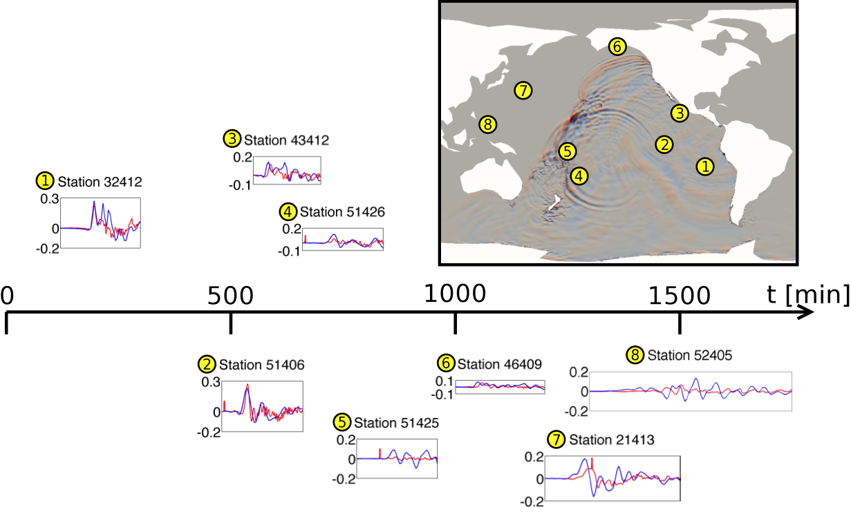
The elevation of the free-surface has been compared with the DART data from the NOAA Center for Tsunami Research at eight different stations. It is seen that the model estimates accurately the time at which the tsunami reaches the different stations. The amplitude of the waves is also well predicted, except for the stations 5 and 8. Those stations being located in very shallow areas with an irregular bathymetry and several small islands, the resolution of the model is probably not sufficient to reproduce accurately the height of the waves.
Free-surface elevation: model data (blue) and DART data (red). The different plot boxes are aligned with the timeline to indicate the time at which the tsunami reaches the different stations (t=0 at the moment of the initial earthquake).
A three-dimensional Discontinuous Galerkin marine model
During my PhD studies, I worked on a three-dimensional Discontinuous Galerkin marine model solving the hydrostatic Boussinesq equations. More information can be found on the model website: SLIM.
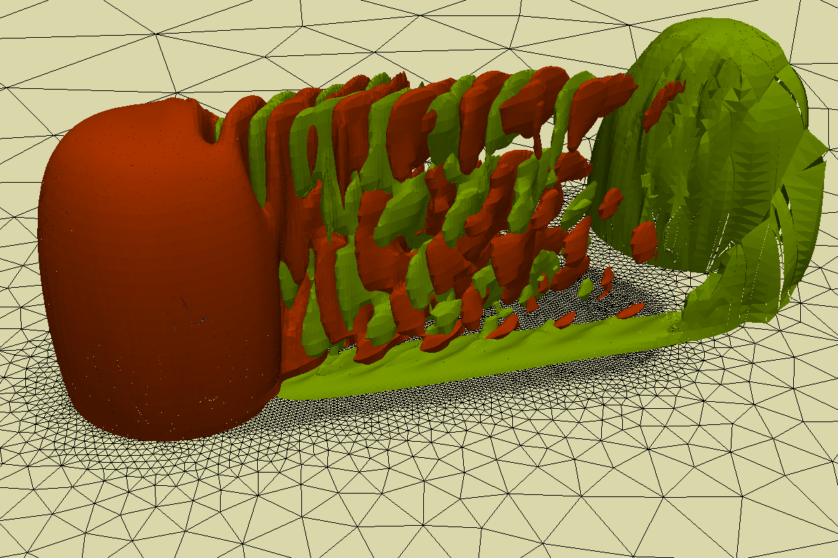
I was in charge of the three-dimensional part of the model. Below is an example of application, showing internal waves generation in the lee of a seamount. To avoid open boundary conditions, the computation is made on the whole sphere, but the mesh is refined only in the area of interest.
Isocontours of density deviation. Isovalues of density deviation are −0.001 kg/m3 in green, and 0.001kg/m3 in red. The two-dimensional mesh, extruded to form the tree-dimensional mesh, is sketched on the sea bottom.